


Skewness tutorials will generally have you do one thing and one thing only: label the tail. Examine the curve. Determine which direction it extends. Label it.
This is not the ability.
What you should know about skewness, when you should attempt to fix it, how, and most importantly, when you shouldn’t touch the data at all is what is important. This tutorial focuses solely on those areas that are often overlooked in any discussion of skewness.
What Will I Learn?
What Is Skewness?
Skewness describes the degree of symmetry within a distribution, more precisely, where its tail lies relative to your data points.
A symmetrical distribution has skewness equal to zero. The normal distribution, also called the bell curve, falls under this category. But not many do.

Data Science Course
Program Highlights
✓ 6 Months Industry-Focused Program
✓ Live Classes by Industry Experts
✓ 15+ Real-World Projects
✓ Resume & Interview Preparation
✓ Placement Assistance
Skills You’ll Build
Python • SQL • Power BI • Statistics • Machine Learning • Generative AI
Left-Skewed Distribution (Negative Skew)
What It Looks Like
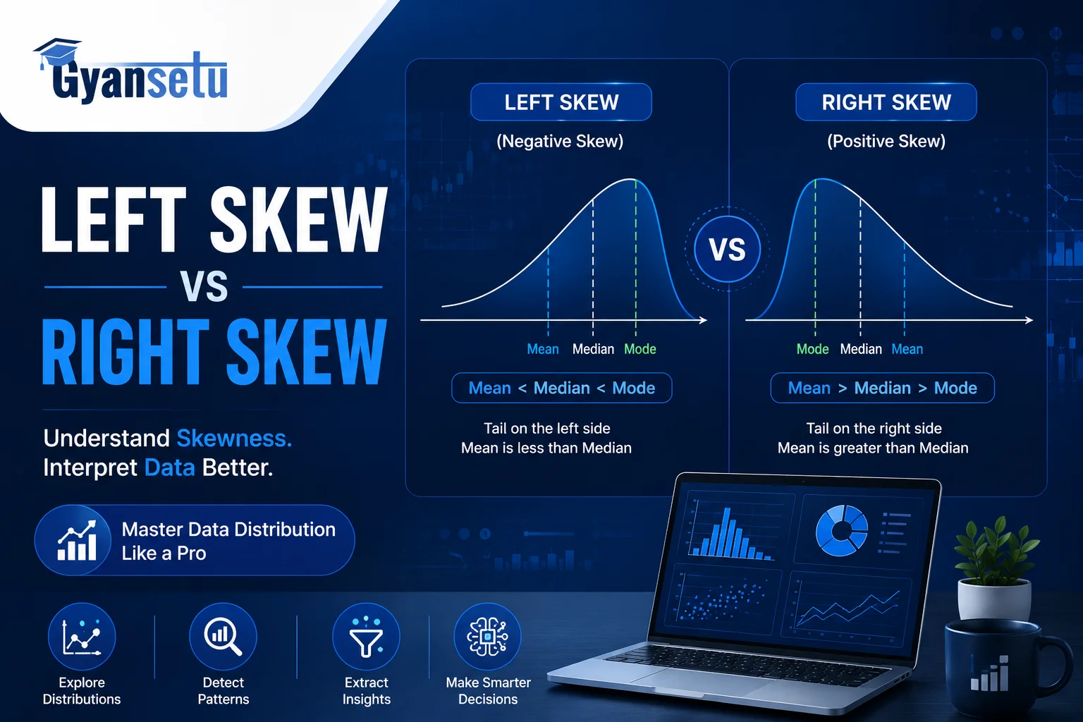
And here is where things get tricky: while the left skewness is characterized by a long tail on the left side, the majority of observations will be concentrated on the right.
The very low values (outliers) will pull the mean to the left, resulting in a normal relationship between Mean, Median, and Mode: Mean < Median < Mode. While the mode will be located at the peak of the curve, the median will be just slightly to the left of the mode.

Real-World Examples of Left Skew
The age of death in developed nations is as follows. Most people live up to their 70s and 80s; some people die young, and the few instances bring the average age of death lower than the actual age of death for the rest.
Here is an example of something related to data science. The precision scores of the folds when using cross-validation on a properly tuned imbalanced classifier tend to be left-skewed. You have precision scores of 0.91, 0.89, and 0.93 on most folds. But you get a precision of 0.61 on one fold. This skews your average precision in a way that a median cannot possibly do.
Right-Skewed Distribution (Positive Skew)

What It Looks Like
Most values fall on the left side. A tail extends to the right. Outliers are much higher than low, hence skewing the mean to be above the median and mode.
Mode < Median < Mean.
In a survey of incomes in a city, one billionaire makes the average income be $340,000 while the median income is $68,000. This $272,000 difference between the average and the median is not an error but right skew in figures.
Real-World Examples of Right Skew
Examples of such distributions include income and price of houses, but there is a better example for those working in ML. The amount of money spent on each purchase in the fraud detection data set usually shows a right-skewed distribution. The majority of legal purchases lie within the range of $5-$200, while a few illegal ones go up to $14,000 or $80,000. Using this raw variable in a logistic regression model will cause your estimates to be biased because the model will give excessive weight to such outliers.
How to Measure Skewness (and What the Numbers Mean)
The Formula
The skewness calculation used in most statistical software is:
Skewness = [n / (n−1)(n−2)] × Σ [(xᵢ − x̄) / s]³
Where n is the number of observations, x̄ is the mean, and s is the standard deviation.
A positive sign indicates a right skew, whereas a negative sign indicates a left skew. The size indicates the extent to which the distribution is skewed. However, in reality, it’s rare to do these calculations manually. More important than the math are the cut-off values, which are not provided in any textbook:
How to Calculate Skewness in Python
Two approaches. Both complete in under five lines.
Using SciPy:
How to Detect Skewness Visually
Three methods. Apply at least one before attempting any transformations.
Histogram:- Draw the graph of your variable. If the big bars are on the right and a long tail hangs out to the left, then the distribution is negatively skewed. Switch around if positively skewed. The graph will show you the asymmetry; the equation will give you the value. You need both, because a skewness value of 0.8 is not the same thing in a sample of 50 observations as in a sample of 50,000.
Box plot:- The line representing the median in the box will move towards one side in case of a skewed distribution. When there is a right skew, the median line will be closer to the bottom of the box, while the top whisker will be much longer than the bottom one.
Q-Q plot:- Surprisingly, it is this technique that most guides tend to omit, and yet it is the most helpful of the three. The Q-Q (quantile-quantile) plot, as described in NIST’s Engineering Statistics Handbook, helps compare the quantiles of your data to those of a normal distribution.
Data that follows a perfect normal distribution will fall along the straight diagonal line. Data that deviates from the norm will form a curve away from the diagonal line, either upwards on the right for positive skew or downwards on the left for negative skew.

How to Fix Skewed Data — Transformations That Actually Work
For Right-Skewed Data
Log Transformation is your first option when values are postitive. The log transform will squish your long right tail well. In truth, if you have values across several orders of magnitude, a log transform is your choice.
Square root transformation is gentler. Good for count data — number of purchases, support tickets, page visits — where the skew exists but isn’t severe.
Box-Cox transformation is the most flexible of the three. It finds the best transformation parameter (lambda) automatically. SciPy handles this:
Use Box-Cox when you’re unsure which specific transform fits best. Let the math decide; that’s what it’s there for.
For Left-Skewed Data
Square transformation emphasizes larger values, bringing the left tail closer to the center. Applicable when all the values are positive, and the skew is not too extreme.
Exponential transformation is even stronger. Apply this transformation when the left tail is extreme, and square transformation does not suffice.
The Yeo-Johnson transformation is the practical choice when dealing with zeros and negative values – scenarios where Box-Cox cannot be used due to its requirement for strictly positive values:
When NOT to Fix Skewness
But most discussions about left skew versus right skew are completely misinformed on this point: they see transformation as the automatic solution when dealing with skewness. It is not.
I’ve seen data scientists spend half a day log-transforming their features for a random forest, doing cross-validation, and achieving virtually identical results while scratching their heads. They did nothing wrong. The transformation simply was unnecessary – and would have been irrespective of how well it addressed the skewness problem.
Models that build decision trees (random forests, gradient boosting, XGBoost, LightGBM) split on thresholds. Their splits do not depend on the shape of the distribution of your feature values. Whether your salary variable follows a bell curve or a hockey stick is irrelevant to your best splits. Transforming your features for such models is extra preprocessing steps without any added value.
Batch-normalized neural networks can cope with skewness in inputs quite well, adjusting the distribution internally at every batch normalization step.
Transform for: linear regression, logistic regression, Naïve Bayes, k-NN, support vector machines.
Do not transform for: random forests, gradient boosting, XGBoost, LightGBM, decision trees.
This decision tree shows precisely which way to go depending on both your skewness score and the kind of model you use.
How Skewness Affects Your Machine Learning Models
The linear regression model requires that the residuals, which are the differences between your predicted value and the actual value, follow a normal distribution. Highly skewed data lead to highly skewed residuals, which go against the assumptions required for the Ordinary Least Squares method, leading to an estimate that is biased and cannot be trusted in terms of statistical reliability.
The Gaussian Naïve Bayes model makes an assumption that all the features are distributed according to the Gaussian distribution within every class. If you provide it with a feature that is skewed beyond 1.5, then the probabilities calculated will be inherently incorrect due to a flawed mathematical assumption made by the model.
Logistic regression is more robust, yet highly skewed features continue to cause issues. The model may end up estimating coefficients based on values that give undue weight to outliers, leading to inaccurate predictions.
Yes, now the other side.
The random forest algorithm does not have any concerns regarding the distribution of features. It simply segments values into categories and does not require knowledge of their form. XGBoost and LightGBM algorithms operate on the same principles. Skewed data is simply not a factor for these algorithms to consider – meaning it is pointless to fix it.
Skewness vs Kurtosis — Quick Distinction
Skewness indicates in which direction your tail lies.
Kurtosis describes whether those tails are thick or thin – but that’s self-explanatory until it’s not. Your distribution can be perfectly symmetrical (skewness = zero), but still be full of extreme outliers in its tails (leptokurtic, high kurtosis) or contain very few outliers in its tails (platykurtic, low kurtosis). Skewness and kurtosis capture two different aspects of the same distribution.

Data Analyst Course
Average time: 6 months
Skills you’ll build: SQL, Python for Data Analysis, Power BI, Excel with AI, Data Storytelling, Stakeholder Reporting
Frequently Asked Questions
Q1. What is the distinction between left skew and right skew?
Ans. In left skew, or negatively skewed, distributions, the tail appears on the left-hand side because the extreme low values make the mean lower than the median. In right skew, or positively skewed distributions, the tail appears on the right side, where extreme high values make the mean higher than the median. The tail always appears on the opposite end from where the bulk of the observations appear.
Q2. How can I tell whether my data is too skewed?
Ans. Apply the following guidelines: A skewness between −0.5 and +0.5 indicates symmetry and is considered acceptable as is. If it is between ±0.5 and ±1.0, then the skewness is moderate. It is better to transform the data in cases beyond ±1.0.
Q3. Which transformation should be used for skewness?
Ans. Log should be applied in case of right skew with positive numbers. Square root can be used if there are counts in the data. If there is any doubt, then apply Box-Cox transformation and optimize the lambda. In case of left skew or presence of zeros or negative numbers, apply Yeo-Johnson.
Q4. Is skewness important for all machine learning algorithms?
Ans. Not necessarily. Random forest, XGBoost, and LightGBM are immune to skewness because their splits are based on threshold logic, not distribution logic. Skewness is important for linear models, logistic regression, Naïve Bayes, k-NN, and SVM. Only fix skewness in those models that are affected by it mathematically.
Q5. What does it indicate when skewness is 0?
Ans. If skewness is zero, then the distribution is symmetrical. Both tails will have the same length and weight. Normal distribution has a theoretical skewness of zero.


