Z-Score Explained

It’s a little-known truth about what’s in your stats book: the z-score equation is easy; figuring out when your solution makes sense isn’t.

Not just a footnote here, either – it’s the entire context of this post. As you read on, you’ll not only learn how to compute z-scores properly but more crucially, how to be sure you’re getting an accurate answer. Something many other tutorials forget to mention completely.

What Is a Z-Score? (The 30-Second Version)

Your physician gives you a lab test result. Your cholesterol is 218 mg/dL. Is there an issue here? You can’t make sense out of this number by itself. For starters, you need to know the average cholesterol in your demographic group and how dispersed the values are within it.

And that’s what a z-score does.

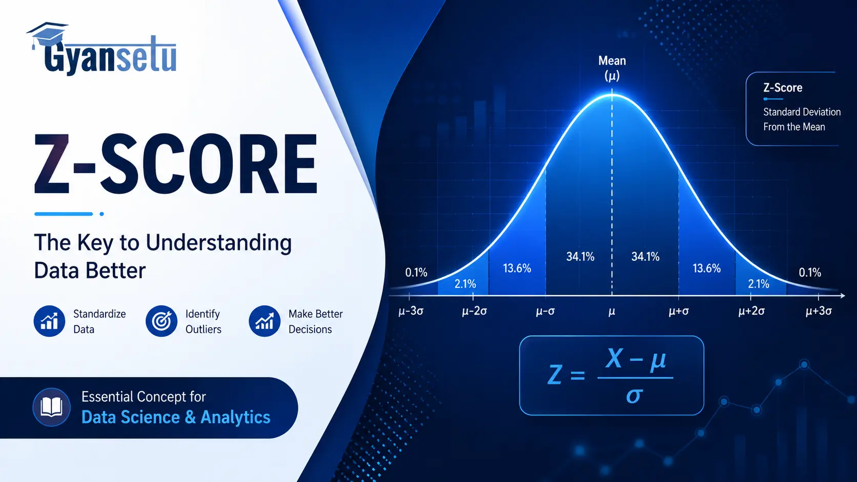
It measures the difference between the value and the mean for its reference distribution measured in standard deviation units. Zero z-score means average value; a z-score of +2 means two standard deviations above the mean, above more than 97.7 percent of values in the reference population. A z-score of −1.5 means below average but nothing extraordinary.

The formula:

In this formula, x represents your raw data point, while μ and σ represent the mean and standard deviation of the population, respectively.

It’s not necessarily the actual z-score formula that makes it worth knowing, since its simplicity may lead one to dismiss it initially. But standardization is the key. The z-score removes the original unit of measurement for comparison purposes, making anything comparable to anything else. This is because now you have a common denominator in terms of the scale.

The Z-Score Formula: Which Version to Use

Three versions exist. Most people learn one. Here’s the thing: picking the wrong one gives you a number that looks legitimate but answers the wrong question.

Version 1: Population z-score

This test should be used when you have the actual population mean and standard deviation beforehand. Standardized tests such as the SAT or even intelligence quotient scales would be considered examples of these. This one uses the given parameters instead of the estimated ones.

Version 2: Sample z-score

Apply this formula when you have raw data that you’ve collected. In this case, x̄ represents the sample mean, and s refers to the sample standard deviation, where n is used in the denominator instead of n−1. It should be noted that using n−1 in the denominator is a correction which is very important but rarely emphasized in introductory statistics.

Version 3: Z-score for a sample mean

Apply this in hypothesis testing, especially when trying to determine if the sample mean is unusually different from the mean of the population. Note that this involves standard error of the mean, which is different from the regular standard deviation.

How to Calculate a Z-Score: Step-by-Step

Here’s a real scenario. You’re reviewing cognitive assessment results for job candidates. The assessment has a population mean of 72 and a standard deviation of 9. One candidate scored 85. Where does that put them?

Step 1: Identify your values. x = 85, μ = 72, σ = 9

Step 2: Subtract the mean. 85 − 72 = 13

Step 3: Divide by the standard deviation. 13 / 9 = 1.44

The Z-score for this candidate is +1.44. The candidate performed 1.44 standard deviations better than the average performance. You can now compare this score directly with that of a candidate who took a totally different test on an entirely different scale.

However, in many cases, one needs to do the opposite. If you have a z-score, you can get the actual score back by reorganizing the equation as follows:

For example, a z-value of −1 indicates (72 + (−1 * 9)) 63. This comes in handy when you have to work in reverse from the percentiles to calculate the cutoff value.

The one less obvious detail here is that if you’re calculating z-scores for an entire set of numbers based on your own data, use Version 2. It will give you slightly wrong results otherwise because you’ll be working with population parameters while sample parameters are needed.

How to Interpret a Z-Score

Positive: above the mean, negative: below the mean. Pretty basic stuff.

This is where the real challenge lies for most of us. Here’s a handy table to keep close by:

Z-Score Range	What It Means	% of Data in This Range
−1 to +1	Within one SD of mean	~68%
−2 to +2	Within two SDs of mean	~95%
−3 to +3	Within three SDs of mean	~99.7%
Beyond ±3	Extremely unusual	< 0.3%

That is the empirical rule. And remember, it works strictly in the case of a normal distribution; that’s an important assumption that isn’t covered well in textbooks. We will see what else can happen next.

There is one particular numerical value which you would find all across your stats book – 1.96. Why do we need it? 1.96 is the borderline, beyond which lies 2.5% of standard normal distribution values, and that makes it the critical value for two-tailed tests at 5% confidence level. But it does not mean that 1.96 is a general cutoff for determining “something is interesting”. It applies only to some specific situations, and its use as the golden line is probably the most prevalent mistake made when applying statistics practically.

To understand why such misconceptions persist, one should realize how widespread they can be. Critical value 1.96 is taught at a beginner level of education and without specifying when this criterion works properly. So chances are that anyone who uses 1.96 as a statistical instrument for decades never knew how it really works.

And just a little note for all those who are scared of zero z-score results. No worries! It just means that the data point is exactly at the average. In clinical measurements, in quality control, in educational assessment being at the mean is often the ideal outcome.

When Z-Scores Break: The Assumptions You’re Probably Ignoring

Take the individual income distribution of a city. Mean: $58,000. Standard deviation: $34,000. Now consider someone with an income of $160,000. His z-score comes out to about 3. Referring to the z-table gives us a percentage figure indicating that he earns more than 99.9% of people in the distribution.

Such reasoning is most likely flawed.

Income distributions tend to be skewed positively. That is because only a few individuals have significantly high incomes and push the average higher and increase the standard deviation. Using this information and referring to a z-table assumes that income distribution follows a normal curve. In real life, that’s not the case. Thus, the value we get from the table isn’t necessarily applicable to this distribution.

I’ve personally experienced how this misconception led to faulty analysis.

The z-score percentile interpretation is valid when two conditions hold:

1. The underlying data is approximately normally distributed — Or if you are applying the Central Limit Theorem to your data, you know for sure that the sampling distribution will be normally distributed as n increases. The generally accepted rule of thumb is when n is greater than 30, but highly skewed populations require even bigger samples.
2. Your parameters are known or reliably estimated — if you’re estimating both the mean and standard deviation from a small sample, additional uncertainty enters the picture that the z-distribution doesn’t account for.

When your data is skewed (financial returns, reaction times, biological measurements, income), you have options:

• Log-transform the data first if it’s right-skewed, then compute z-scores on the transformed values. This works well for income, prices, and other quantities that can’t be negative.
• Use Chebyshev’s theorem for a distribution-free probability bound. It guarantees that at least 75% of any dataset, regardless of shape, falls within 2 standard deviations of the mean. The estimates are conservative; they don’t require normality.
• Switch to a t-score when your sample is small and the population standard deviation is unknown.

Most z-score articles get this exactly wrong: they present the formula as sufficient, treat the z-table as universally applicable, and leave readers with a tool that quietly breaks in the most common real-world conditions. The formula is simple; the judgment about when to use it is not.

How to Use the Z-Table

The z-table takes the z-score and finds the cumulative probability for the area below that score in a standard normal distribution.

Using the z-table involves looking up two coordinates. The integer portion and the tenths digit of the z-score go down the vertical axis on the left side, while the hundredths digit goes along the horizontal axis at the top.

Example: z-score of 1.44. Locate 1.4 down the left column. Then find 0.04 along the top row. Their intersection is the cumulative probability of 0.9251.

It tells you that 92.51 percent of the data lie to the left of a z-score of 1.44. Hence, the candidate’s score is above 92 percent of the reference group.

Most tables also have symmetric entries for the z-table values. Thus, a z-score of -1.44 will give a cumulative probability of 0.0749. To check, 0.0749+0.9251 = 1.00.

In other words, 7.5 percent of the data lie below that score. To get the area between two z-scores, just look up both probabilities and take the difference.

In 2026, most analysts will use a calculator or statistical software rather than a printed table. That’s fine. But working through the table at least once teaches the underlying logic in a way that typing into a function does not, and that understanding matters when you need to explain a result to someone who doesn’t already trust your output.

How to Calculate Z-Scores in Excel, Python, and R

Excel

The STANDARDIZE() function handles it directly:

=STANDARDIZE(x, mean, standard_dev)

For the candidate example: =STANDARDIZE(85, 72, 9) returns 1.44.

To standardize a full column, calculate the mean with AVERAGE() and the standard deviation with either STDEV.P() (population data) or STDEV.S() (sample data), then reference those cells inside your STANDARDIZE formula and copy it down the column.

Python

python
import numpy as np
from scipy import stats

scores = np.array([85, 72, 68, 90, 77])

# Population z-scores (divides by N, not N-1)
z_scores = stats.zscore(scores)
print(z_scores)

# Manual calculation -- explicit control over ddof
mean = np.mean(scores)
std = np.std(scores, ddof=0)  # ddof=0 = population SD
z_manual = (scores - mean) / std
print(z_manual)

One thing worth flagging explicitly, because it trips people up when comparing output across languages: scipy.stats.zscore() uses population standard deviation (ddof=0) by default. R’s scale() uses sample standard deviation (ddof=1). On large datasets the difference is negligible; on small samples it compounds. Check which denominator each tool is using before you trust a cross-language comparison.

R

r
scores <- c(85, 72, 68, 90, 77)

# scale() uses sample SD (ddof=1) by default
z_scores <- scale(scores)[, 1]
print(z_scores)

For machine learning preprocessing, Python’s sklearn.preprocessing.StandardScaler is the standard tool for z-score standardization. Its fit/transform pattern matters: fit the scaler on training data only, then apply the same fitted scaler to test data. Fitting on the full dataset before the train/test split leaks test information into the scaling parameters — a subtle error that inflates performance metrics in ways that are easy to miss.

Z-Scores in the Real World: 5 Applications That Actually Matter

1. Outlier Detection in Data Pipelines

A z-score threshold of ±3 is the most common first-pass outlier filter in data cleaning. Any data point beyond three standard deviations gets flagged for review. It’s not infallible — a legitimate extreme value can cross that threshold — but it’s fast, transparent, and defensible.

python
outlier_mask = np.abs(z_scores) > 3
clean_data = data[~outlier_mask]

What makes this useful in preprocessing: it’s scale-invariant. You can apply it uniformly across all features in a dataset without knowing each feature’s original units.

2. The Altman Z-Score (A Completely Different Animal)

However, if your point of origin is within the realm of finance, you might want information that is missing in this particular article. The Z-Score of Altman, developed by NYU’s Edward Altman in 1968, determines the probability of an organization falling into bankruptcy within two years. It is said that Altman initially tried to measure as many as 22 financial ratios before he finally settled for five: working capital /total assets, retained earnings/total assets, EBIT/total assets, market value of equity/book value of liabilities, and sales/total assets.

The Altman Z-Score has the same name as the statistical z-score. No relation between the two at all. Just wanted to clarify this from the start so as not to mislead anyone.

3. Child Growth Charts and WHO Standards

Z-scores can be used by pediatricians in child development assessment. Any z-score below −2 is the clinical criterion for stunting among children under the WHO growth standards. Nutrition programs around the world utilize the criterion for identifying children requiring direct intervention.

If a doctor states that a child has reached the 5th percentile mark in height, it simply means that the doctor is applying z-score thinking along a differently scaled axis. It’s the same math used in this article.

4. Standardized Testing and IQ Scores

The IQ score scale has been set to have a mean score of 100 and a standard deviation of 15 points. The IQ score can be likened to the z-score only that in this case the normal curve has been shifted and expanded. For instance, an IQ score of 130 is a score of +2 (the 97.7th percentile).

5. Six Sigma and Quality Control

The Six Sigma manufacturing system operates solely on z score principles. The concept “Six Sigma” implies that the closest specification lies six standard deviations away from the process mean, or in other words, there will be only 3.4 defects per one million opportunities. Control charts utilize ±3σ as control limits, whereby an observation that exceeds this range is an indication for investigation of the process.

Z-Score vs T-Score: Which One Do You Need?

The short answer is: use a z-score when you know the population standard deviation and your sample is large enough (n > 30 is the standard threshold). Use a t-score otherwise.

Here’s why the distinction matters. When you estimate the standard deviation from your own data, which is almost always what you’re doing in practice, that estimate carries uncertainty. The t-distribution accounts for that uncertainty through a parameter called degrees of freedom. The smaller your sample, the heavier the tails of the t-distribution, and the more extreme a result needs to be before you flag it as unusual. As n grows, the t-distribution converges to the normal distribution. At n = 200, the two tests give nearly identical results.

Practically: if you’re running a one-sample test with n = 12, use a t-test. With n = 300 and roughly normal data, z and t produce the same answer.

One important clarification for medical readers. In bone density testing, doctors interpret both T-scores and Z-scores, but these are not the same as statistical t-scores and z-scores. The bone density T-score compares your bone density to a healthy young adult reference population; the bone density Z-score compares it to age-matched peers. The naming overlap with statistical tools causes genuine confusion in practice. They are distinct clinical metrics.

Frequently Asked Questions

Closing

It’s easy to calculate the numbers. The difficulty lies in deciding whether you even have a right to interpret your data within the context of a normal distribution. If you make that determination correctly, you will be using z-scores far more responsibly and properly than the majority of those running them daily.