Skewness and Kurtosis

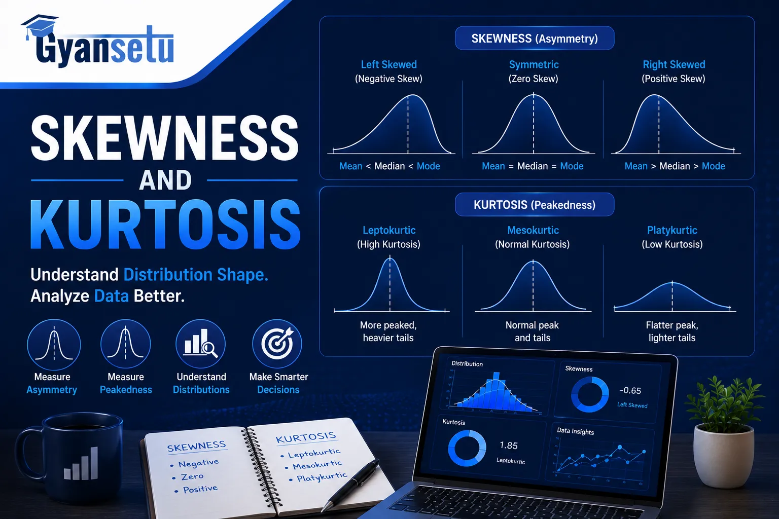
Typically, most tutorials cover skewness and kurtosis by defining them. Learn the definition, know the form, answer the questions right. This approach is wrong because most data science projects fall apart due to data that does not cooperate in line with textbook distributions.

Skewness and kurtosis are decision points. Skewness helps you understand if your data is tilting towards a specific direction. On the other hand, kurtosis will help you understand if the outliers are causing the issue. Both will help you move to the next step. This article highlights everything about skewness and kurtosis, including calculations in Python and what comes after.

Quick-Reference: Skewness vs. Kurtosis at a Glance

	Skewness	Kurtosis
What it measures	Directional asymmetry (which tail is longer)	Tail weight (how much data lives in the extremes)
Formula type	3rd moment	4th moment
Normal distribution value	0	3 (excess kurtosis = 0)
Python — pandas	df[‘col’].skew()	df[‘col’].kurt()
Python — scipy	scipy.stats.skew(x)	scipy.stats.kurtosis(x)
“Normal enough” threshold	Between −0.5 and +0.5	Excess kurtosis between −1 and +1
Action when high	Consider log, sqrt, or power transform	Investigate outliers first; transform if needed

What Skewness Actually Measures (And What It Doesn’t)

Here is the misconception that the beginners hold about skewness. It does not represent the direction of the tail but rather its location. The peak is located on the opposite side from the tail. With right skewness, most observations will be on the left side, with the tail stretching towards the right and pushing the mean upwards.

The idea originated in the work of Karl Pearson in the beginning of the 20th century, when the language of probability distributions was being created. Skewness did not become standardized before 1895.

Right Skew (Positive Skewness)

Another practical example would be insurance claims. Most of the claims tend to be low, such as a damaged windscreen or a slight fender bender. However, every once in a while, there is going to be a massive claim, and this will shift the mean well above the range of what the majority of policyholders usually claim. The tail stretches to the right; the bulk remains to the left.

With the right-skewed curve: mean > median > mode.

The mean is influenced by the tail effect. However, the median will resist this tendency, which is why real estate agents report the median values of homes for sale rather than the mean values. One home selling at $40 million will not represent the neighborhood!

Left Skew (Negative Skewness)

Flip the scenario around. Consider test scores for an easy test, where almost all the students got scores ranging from 85 to 100. A small group of those who did not prepare for the test scored close to 0. These few will shift the mean towards the left side of the graph.

In a left-skewed distribution: mean < median < mode.

Zero Skewness, When It Lies

But this is what most articles leave out. Zero skewness doesn’t indicate that your data follows a normal distribution. What it tells you is that your data distribution is symmetric… but not necessarily normally distributed.

Zero skewness is seen in a t-distribution with fewer degrees of freedom. The t-distribution here is perfectly symmetric. But because of the heavy tails, any model built using the t-distribution results in invalid confidence intervals. And if you see a situation where zero skewness coexists with high kurtosis, then you know for sure that this isn’t a case to be treated as “looks good, proceed.”

The key point: skewness indicates only the direction of deviation.

The Skewness Formula, Three Ways to Calculate It

Pearson’s Second Coefficient (The Quick One)

The simplest formula:

Skewness = 3 × (mean − median) / standard deviation

This is called the median skewness, or Pearson’s second coefficient. Fast, interpretable, and gives you a directional signal immediately. The numerator captures how far the mean has been pulled from the median, which is exactly what skewness represents conceptually.

python
import numpy as np
import seaborn as sns

diamonds = sns.load_dataset("diamonds")
prices = diamonds["price"]

mean_price   = prices.mean()
median_price = prices.median()
std_price    = prices.std()

pearson_skew = 3 * (mean_price - median_price) / std_price
print(f"Pearson's 2nd coefficient: {pearson_skew:.4f}")
# Output: 1.1519

Moment-Based Formula (The Rigorous One)

The standard formula used by most software is the Fisher-Pearson coefficient, the third standardized moment:

g₁ = [n / ((n−1)(n−2))] × Σ[(xᵢ − x̄) / s]³

The n / ((n−1)(n−2)) term is a bias correction for sample size. For large datasets, it barely moves the needle. For small ones (a 40-row clinical trial, a 25-observation pilot study) it shifts the estimate noticeably. Worth knowing.

python
def moment_skewness(x):
    n    = len(x)
    mean = np.mean(x)
    std  = np.std(x)
    adj  = n / ((n - 1) * (n - 2))
    core = np.sum(((x - mean) / std) ** 3)
    return adj * core

print(f"Moment-based skewness: {moment_skewness(prices):.4f}")
# Output: 1.6184

Python Shortcut, pandas, scipy, and Why They Disagree

Run both libraries on the same data and you’ll get different numbers from Pearson’s formula. That’s not a bug; it’s a different formula.

python
from scipy.stats import skew

print(f"pandas .skew():      {prices.skew():.4f}")   # 1.6184
print(f"scipy skew():        {skew(prices):.4f}")    # 1.6184
print(f"Pearson's 2nd:       {pearson_skew:.4f}")    # 1.1519

pandas and scipy agree here because both use the adjusted Fisher-Pearson formula. Pearson’s second coefficient gives a lower number because it’s a different formula: not wrong, just measuring something slightly different. Neither answer is incorrect. They’re answering different versions of the same question.

Takeaway: for EDA and machine learning workflows, pandas .skew() is the standard. Pearson’s second coefficient is useful for quick sanity checks.

Interpreting Your Skewness Score, The Thresholds That Actually Matter

The widely used thresholds come from applied statistical guidance:

Score Range	Classification	Action
−0.5 to +0.5	Approximately symmetric	Parametric tests generally fine; no transformation needed
±0.5 to ±1	Moderately skewed	Check algorithm sensitivity; linear models may need a transform
Beyond ±1	Highly skewed	Transform before linear modeling; tree models typically unaffected

One thing the benchmarks don’t say: context changes the threshold. A skewness of 0.8 in a 500,000-row transaction log is probably fine. The same score in a 40-row clinical study warrants more scrutiny, because the skewness estimate itself is noisier with small samples.

What Kurtosis Actually Measures, The Tail Weight vs. Peak Debate

Textbooks generally define kurtosis as a measure of peakedness. This approach is erroneous or at the very least deceptive.

Peter Westfall in his work “Kurtosis as Peakedness, 1905–2014. R.I.P.” which was published in 2014 in The American Statistician proves that the shape of a probability distribution does not tell us anything about its peakedness; one can find the distribution having a highly pointed (needle-like) peak but still having almost no kurtosis, and vice versa – completely unpeaked (completely flat-top) distribution may have kurtosis close to infinity. The definition is disproved by mathematics immediately.

Kurtosis is actually a measure of tail weight. It shows how many observations in your sample fall into extremes compared to the normal distribution. If the kurtosis value is high, the number of observations falling into extremes is high.

The Three Types of Kurtosis

Mesokurtic (excess kurtosis ≈ 0): Tails similar to a normal distribution. Most controlled experimental data lands here when conditions are stable.

Leptokurtic (excess kurtosis > 0): Fat tails, more extreme values than normal. Daily equity returns are almost universally leptokurtic — the “five-sigma event happens far too often” problem that broke several quantitative hedge fund models in 2008. 

Platykurtic (excess kurtosis < 0): Thin tails, fewer extreme values. A uniform distribution is platykurtic. The outcomes are bounded, so genuinely extreme results can’t occur.

Kurtosis vs. Excess Kurtosis, The Confusion Explained

A normal distribution has a raw kurtosis of 3. That’s an inconvenient baseline, so statisticians subtract 3 to create excess kurtosis, which recenters normal at zero.

Excess kurtosis = Raw kurtosis − 3

pandas .kurt() returns excess kurtosis. scipy’s kurtosis() also returns excess kurtosis by default. But older textbooks and the NIST Handbook report raw kurtosis, where normal equals 3, not 0. When a colleague says “the kurtosis is 5.9,” ask which convention they’re using. The conclusion changes.

Takeaway: in Python, assume excess kurtosis unless explicitly told otherwise. Normal = 0, not 3.

Calculating Kurtosis in Python, With the Libraries You’re Already Using

python
from scipy.stats import kurtosis
import pandas as pd
import numpy as np

prices = diamonds["price"]

# Excess kurtosis (normal = 0)
print(f"pandas kurt():              {prices.kurt():.4f}")             # 2.1777
print(f"scipy kurtosis():           {kurtosis(prices):.4f}")          # 2.1774

# Raw kurtosis (normal = 3)
print(f"scipy raw kurtosis:         {kurtosis(prices, fisher=False):.4f}")  # 5.1774

# Manual excess kurtosis
n     = len(prices)
mean  = np.mean(prices)
std   = np.std(prices)
manual = (1/n) * np.sum(((prices - mean) / std) ** 4) - 3
print(f"Manual excess kurtosis:     {manual:.4f}")                    # 2.1774

The small gap between pandas and scipy comes from different bias correction formulas. For 50,000+ rows, it’s noise.For a 30-row sample, compare them explicitly before reporting either number.

Reading Skewness and Kurtosis Together, The Joint Interpretation Skill

This is the most useful section in the article. And it exists nowhere in the current top-10 search results.

Skewness and kurtosis don’t simply add up, they interact. The combination tells you more than either number alone. There are four patterns you’ll encounter in real data:

Low skewness + low kurtosis → Close to normal. Parametric tests are safe. Proceed to modeling without transformation.

Low skewness + high kurtosis → Symmetric but fat-tailed. This is an outlier problem, not a skewness problem. Transforming the data won’t help much. The right move is to investigate where the extreme values come from — are they real events, sensor errors, or data entry mistakes?

High skewness + low kurtosis → Data leans in one direction, but the extremes aren’t especially heavy. A log or square root transform usually resolves this. Tree-based models may not need it at all.

High skewness + high kurtosis → Both issues present simultaneously. Don’t rush to transform. Check the domain first. Income data looks like this by design — and transforming it to look normal can strip out economically meaningful signal.

Why This Matters for Machine Learning, The Algorithm Impact Guide

Honestly, I’ve watched this happen more than once: a team log-transforms every skewed feature reflexively, then wonders why their random forest’s accuracy didn’t budge. Tree-based models don’t care about input distributions. You added complexity and lost nothing, except interpretability.

The table below is what actually determines whether transformation is worth doing:

Algorithm	Skewness Sensitive	Kurtosis Sensitive	Notes
Linear Regression	✅ Yes	✅ Yes	OLS estimates stay unbiased; confidence intervals degrade
Logistic Regression	✅ Moderate	✅ Moderate	Convergence slows; probability estimates at extremes become unreliable
Decision Tree / Random Forest	❌ No	❌ No	Threshold splits; distribution shape is irrelevant to the algorithm
SVM (RBF kernel)	✅ Moderate	✅ Yes	Outlier-sensitive kernels are affected by fat-tail behavior
Neural Networks	⚠️ Depends	⚠️ Depends	High kurtosis can cause gradient instability without input normalization
KNN	✅ Yes	✅ Yes	Distance calculations are distorted by extreme values
Gaussian Naive Bayes	✅ Yes	❌ Minimal	Explicitly assumes normally distributed features

Takeaway: knowing which row of this table applies to your project is more valuable than memorizing any skewness formula.

What To Do About Skewness and Kurtosis, Transformations That Work

Log Transform, When and Why

Best use case: right-skewed data where every value is strictly positive. Income, transaction amounts, user session counts, classic candidates.

python
import numpy as np

log_prices = np.log1p(prices)   # log1p = log(1 + x); handles zeros safely

print(f"Original skewness:  {prices.skew():.4f}")      # 1.6184
print(f"Log skewness:       {log_prices.skew():.4f}")  # 0.3879

Use np.log1p() instead of np.log() whenever zeros are possible. log(0) is undefined; log1p(0) returns 0. Small detail that prevents a runtime error in production.

Square Root Transform

Milder than log. Good for counting data with moderate right skew, support ticket volumes, page views per session. When the log transform overcorrects and produces left skew, try square root first.

python
sqrt_prices = np.sqrt(prices)
print(f"Sqrt skewness:  {sqrt_prices.skew():.4f}")  # 0.9356

Still skewed, but less so. If 0.9 is close enough to your threshold for the algorithm you’re using, square root is the simpler, more interpretable choice.

Box-Cox Transform

Box-Cox is the general parametric approach. It searches for the power lambda (λ) that best normalizes your data, so you don’t have to guess whether log, square root, or cube root is right.

python
from scipy.stats import boxcox
import pandas as pd

bc_values, lambda_val = boxcox(prices)
bc_series = pd.Series(bc_values)

print(f"Optimal lambda:     {lambda_val:.4f}")
print(f"Box-Cox skewness:   {bc_series.skew():.4f}")

One hard constraint: Box-Cox only works on strictly positive values. If your column contains zeros or negative numbers, it raises an error. That’s where Yeo-Johnson comes in.

Yeo-Johnson Transform, The Modern Choice

Yeo-Johnson is Box-Cox without the positivity requirement. It handles zeros and negative values, and it’s what scikit-learn’s PowerTransformer uses by default.

python
from sklearn.preprocessing import PowerTransformer
import pandas as pd

pt = PowerTransformer(method='yeo-johnson')   # default
transformed = pt.fit_transform(prices.values.reshape(-1, 1))
yj_series   = pd.Series(transformed.flatten())

print(f"Yeo-Johnson skewness:  {yj_series.skew():.4f}")

If you’re building scikit-learn pipelines, this is the right tool. It integrates with Pipeline, supports inverse_transform() for interpretability, and works across the full range of real numbers.

When NOT to Transform

Three situations where transformation is the wrong move, and skipping it is the right call:

Your model is tree-based. Decision trees, random forests, XGBoost, and LightGBM don’t care about the shape of input distributions. Transforming features before these models adds complexity with no performance benefit. The splits adapt to whatever values are present.

The skewness is structurally real. Income is right-skewed because that’s how income distributes across populations. If you log-transform it, then later need to explain model outputs to a business stakeholder, you’ve created an interpretation problem for no modeling gain. The skewness was information, not noise.

You have symmetric data with negative excess kurtosis. Platykurtic symmetric data doesn’t need transformation. It’s more uniform than normal — and that’s fine for most algorithms.

Takeaway: always ask “which algorithm am I using?” before reaching for a transformation. The algorithm question answers the transformation question.

Visualizing Skewness and Kurtosis, The Right Charts

KDE Plot with Annotations (Seaborn)

A kernel density estimate plot shows distribution shape without the bin-count decisions that make histograms finicky. Add vertical lines for mean, median, and mode to make the skewness visible.

python
import matplotlib.pyplot as plt
import seaborn as sns

fig, ax = plt.subplots(figsize=(10, 5))
sns.kdeplot(prices, ax=ax, color='steelblue', linewidth=2)

ax.axvline(prices.mean(),    color='red',   linestyle='--',
          label=f'Mean ({prices.mean():.0f})')
ax.axvline(prices.median(),  color='black', linestyle='--',
          label=f'Median ({prices.median():.0f})')
ax.axvline(prices.mode()[0], color='green', linestyle='--',
          label=f'Mode ({prices.mode()[0]:.0f})')

sns.despine(top=True, right=True, left=True, ax=ax)
ax.set_title(f'Diamond Prices, Skewness: {prices.skew():.2f}', fontsize=14)
ax.legend()
plt.tight_layout()
plt.show()

The gap between mean and median tells the story before you read the skewness number. When the mean sits visibly to the right of the median, you’re looking at a right-skewed distribution.

Histogram + KDE Overlay

When you want both raw counts and the smoothed shape in one view:

python
sns.histplot(prices, bins=40, kde=True,
            kde_kws={'bw_adjust': 2},
            color='steelblue', alpha=0.6)

plt.title('Diamond Prices, Histogram with KDE Overlay')
plt.xlabel('Price ($)')
plt.show()

bw_adjust controls smoothness. Values above 1 smooth out local spikes; below 1 reveals more granular variation. For EDA, a value between 1.5 and 2.5 usually produces the clearest shape signal.

QQ Plot for Normality Assessment

A quantile-quantile (QQ) plot puts your data’s quantiles on one axis and theoretical normal quantiles on the other. Points on the diagonal line = approximately normal. Deviations reveal both skewness and kurtosis at a glance.

python
from scipy import stats

fig, ax = plt.subplots(figsize=(6, 6))
stats.probplot(prices, plot=ax)
ax.set_title('QQ Plot, Diamond Prices')
plt.tight_layout()
plt.show()

Right skewness shows up as an upward curve at the right end. High kurtosis produces an S-shaped deviation at both ends, where tails lift away from the diagonal line. One chart, two signals; the most information-dense diagnostic in a standard EDA toolkit.

Frequently Asked Questions