SARSA in Reinforcement Learning

Q-learning finds the optimal path to the destination point. Then it proceeds to move along the cliff edge and falls off the cliff 30 percent of the time. The SARSA algorithm prefers a longer way of travel. More secure territory. Make it safely 100 percent of the time. And this single behavioral difference – rather than anything else: the mathematics behind, the coding, the equation – is why the SARSA algorithm exists. All the tutorials you’ve ever read started out with the expanded meaning of the acronym and the famous Bellman equation. This tutorial begins here because once you understand the motivation behind SARSA, everything else will come naturally.

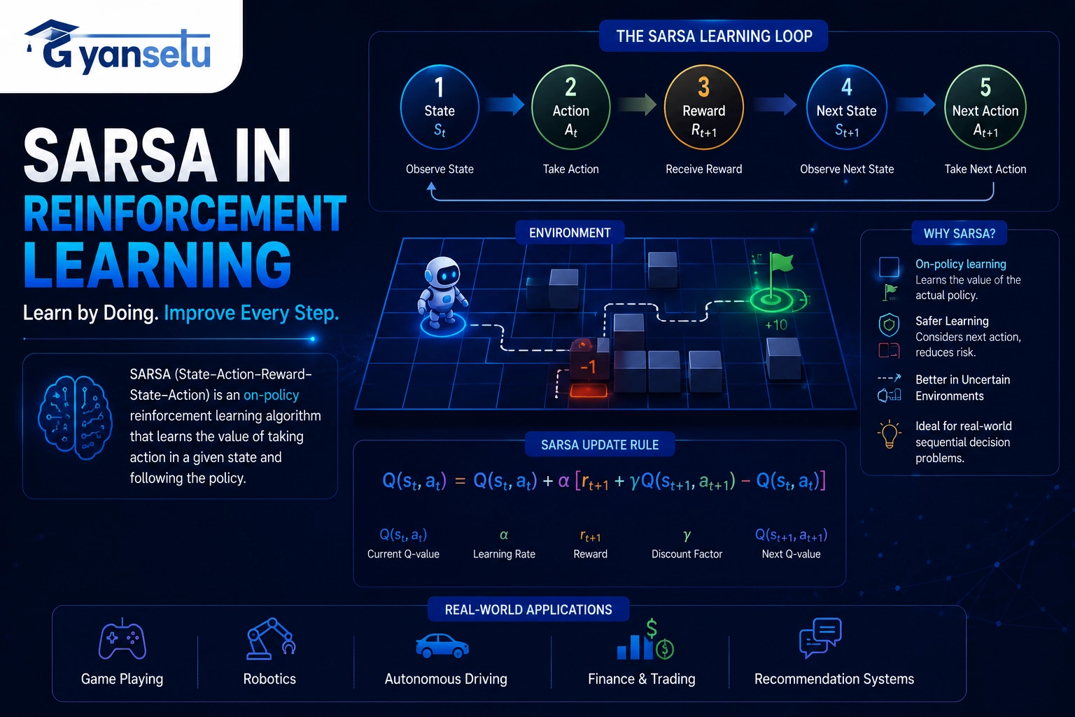
SARSA is an on-policy reinforcement learning algorithm, in which the Q-values are calculated according to the action that was actually taken, and not the action that theoretically would have led to the maximum reward. The acronym means State-Action-Reward-State-Action – the five factors involved in the update. The algorithm was first introduced in 1994 by Rummery and Niranjan, and then gained popularity in Sutton and Barto’s Reinforcement Learning: An Introduction.

By the end of this article you’ll understand how the update rule works, how to run SARSA in Python using Gymnasium, why it learns safer behavior than Q-learning, and when you should actually pick it for a real project.

What Is SARSA?

SARSA is an on-policy RL algorithm, one that learns the value of the current policy being followed by the agent, inclusive of its exploration steps.

And the key point here is that last part. Most RL algorithms keep the actions taken by the agent while training different from the actions it takes later on. But not SARSA. In SARSA, whenever the agent takes an exploration step (by taking a random action), it gets included in the algorithm. The outcome is an agent that knows the risks.

The five components of SARSA

Every SARSA update uses exactly five pieces of information. Here’s what each one means in plain terms:

Component	Symbol	What It Means
State	S	Where the agent is right now (e.g., the room the robot is currently in)
Action	A	What the agent does in that state (e.g., move left)
Reward	R	The feedback it gets immediately after acting (e.g., +10 for reaching the goal)
Next State	S’	Where the agent ends up after the action (e.g., the next room)
Next Action	A’	What the agent does next, chosen by the same policy (e.g., move right)

And that very column, A’, which denotes the next action, is what distinguishes SARSA from Q-learning. Q-learning updates the value using the optimal next action, but SARSA updates the value based on the next action that is actually taken by the agent. If this is an exploratory move chosen randomly, then that too would be accounted for.

This is why SARSA is named SARSA, i.e., the tuple (S, A, R, S’, A’).

How the SARSA Update Rule Works

The formula looks more intimidating than it is:

Q(S, A) ← Q(S, A) + α [ R + γ · Q(S’, A’) − Q(S, A) ]

Here’s what each piece means in everyday language:

• Q(S, A) — Your best guess as to how good it is to take action A in state S
• α (alpha) — How quickly your belief is updated; alpha = 0 ignores any new information, while alpha = 1 considers only the most recent experience.
• R — the reward you just got
• γ (gamma) — How much you discount the future; the closer gamma is to 1, the more you consider the long-term, and vice versa.
• Q(S’, A’) — your best guess as to the next situation.
• The bracketed term — the temporal difference (TD) error, which indicates your level of surprise.

This is where it gets exciting: prior to taking the action, you had some expectations. Afterwards, you learned what actually occurred. The difference between these two values is the TD error. It becomes positive whenever the outcome is better than anticipated, causing Q(S, A) to increase. When the result is worse, Q(S, A) decreases. Zero indicates your model is accurate.

After thousands of such updates, through many episodes, the Q-values converge on an accurate representation of the world.

Step by step: what happens in a single SARSA update

• Agent finds itself at state S and selects an action A as per its current policy (usually epsilon-greedy policy)
• Action is performed, and agent gets a reward R along with reaching state S‘
• Agent immediately selects its next action A’ from S’ – again following the same epsilon-greedy policy
• These five figures are substituted in the equation above for update
• It reaches state S’, and A’ is considered as the new A for the next iteration

It is this step 3 that makes the SARSA algorithm on-policy.

Implementing SARSA in Python

The Taxi-v3 Gymnasium environment will be used. In this problem, a taxi travels around the 5×5 grid to pick up passengers from four different locations and deliver them to their desired location. If a correct passenger is picked up and successfully delivered, a reward of +20 is given, and a -10 reward is given if the pickup and delivery are illegal. 

First, install the Gymnasium library:

bash

pip install gymnasium

Setting up the environment and Q-table

python

import gymnasium as gym

import numpy as np

import matplotlib.pyplot as plt

def create_environment(env_name="Taxi-v3"):

    return gym.make(env_name, render_mode="rgb_array")

def initialize_q_table(env):

    n_states = env.observation_space.n   # 500 for Taxi-v3

    n_actions = env.action_space.n       # 6 for Taxi-v3

    return np.zeros((n_states, n_actions))

Start with all Q-values at zero. The agent knows nothing yet.

The epsilon-greedy policy

python

def epsilon_greedy(env, Q_table, state, epsilon):

    # With probability epsilon: explore (random action)

    if np.random.random() < epsilon:

        return env.action_space.sample()

    # Otherwise: exploit (best known action)

    return np.argmax(Q_table[state])

Epsilon controls the explore/exploit balance. At ε = 0.1, the agent explores 10% of the time.

Epsilon decay — the part most tutorials skip

This is what is wrong with leaving the epsilon value at 0.1 indefinitely: the agent will not learn to stick to what it knows. In the early episodes, exploration is necessary. However, in episode 15,000, the agent will have seen everything it could — exploration is pointless now.

Exponential decay fixes this:

python

def get_epsilon(episode, epsilon_start=1.0, epsilon_end=0.01, decay_rate=0.001):

    return epsilon_end + (epsilon_start - epsilon_end) * np.exp(-decay_rate * episode)

Linear decay is simpler but cruder:

python

def get_epsilon_linear(episode, total_episodes, epsilon_start=1.0, epsilon_end=0.01):

    fraction = min(episode / total_episodes, 1.0)

    return epsilon_start + fraction * (epsilon_end - epsilon_start)

Exponential decay drops fast early and slows down near zero — which matches how learning actually progresses. Use it.

The SARSA update rule

python

def sarsa_update(Q_table, state, action, reward, next_state, next_action, alpha, gamma):

    current_q = Q_table[state, action]

    next_q = Q_table[next_state, next_action]

    td_error = reward + gamma * next_q - current_q

    Q_table[state, action] += alpha * td_error

The full training loop

python

def train_sarsa(env, n_episodes=20000, alpha=0.1, gamma=0.99,

                epsilon_start=1.0, epsilon_end=0.01, decay_rate=0.001):

    Q_table = initialize_q_table(env)

    episode_rewards = []

    episode_lengths = []

    for episode in range(n_episodes):

        state, _ = env.reset()

        epsilon = get_epsilon(episode, epsilon_start, epsilon_end, decay_rate)

        action = epsilon_greedy(env, Q_table, state, epsilon)

        done = False

        total_reward = 0

        steps = 0

        while not done:

            next_state, reward, terminated, truncated, _ = env.step(action)

            done = terminated or truncated

            next_action = epsilon_greedy(env, Q_table, next_state, epsilon)

            sarsa_update(Q_table, state, action, reward, next_state, next_action, alpha, gamma)

            state = next_state

            action = next_action

            total_reward += reward

            steps += 1

        episode_rewards.append(total_reward)

        episode_lengths.append(steps)

        if episode % 2000 == 0:

            avg_r = np.mean(episode_rewards[-1000:])

            print(f"Episode {episode:>6} | Avg reward (last 1000): {avg_r:.2f} | ε: {epsilon:.3f}")

    return Q_table, episode_rewards, episode_lengths

Notice: next_action is chosen before the update, using the same epsilon from the current episode. That’s on-policy behavior.

Running it

python

env = create_environment()

Q_table, rewards, lengths = train_sarsa(env, n_episodes=20000)

# Plot learning curve

plt.figure(figsize=(12, 4))

plt.subplot(1, 2, 1)

plt.plot(rewards)

plt.title("Episode rewards")

plt.xlabel("Episode")

plt.subplot(1, 2, 2)

plt.plot(lengths)

plt.title("Episode lengths (steps)")

plt.xlabel("Episode")

plt.tight_layout()

plt.show()

You’ll see rewards start deeply negative (around -500) and stabilize around +7 to +10 after roughly 5,000 episodes. Episode lengths drop from 200 (the max) to around 13–16 steps. That’s a working SARSA agent.

SARSA vs Q-Learning — The Real Difference

The formulas differ by exactly one word.

SARSA: Q(S, A) ← Q(S, A) + α [ R + γ · Q(S’, A’) − Q(S, A) ]

Q-learning: Q(S, A) ← Q(S, A) + α [ R + γ · max Q(S’, a) − Q(S, A) ]

Q-learning always assumes the agent will take the best action next. SARSA assumes the agent will take the actual action next — which might be a random exploratory move.

Feature	SARSA (on-policy)	Q-learning (off-policy)
Update target	Q-value of the action actually taken	Maximum Q-value of the next state
Policy type	On-policy — learns the value of the policy it follows	Off-policy — learns the optimal policy regardless of behavior
Behavior in risky environments	Conservative; accounts for exploratory mistakes	Aggressive; ignores exploration noise
Convergence speed	Slower	Faster
Final policy quality	Near-optimal (bounded by exploration)	Optimal (in the limit)
Best environment type	Stochastic, risky, or costly to explore	Simulated, resets are free, exploration is cheap

The cliff-walking proof

Sutton and Barto’s cliff-walking example is the clearest demonstration of this difference, and I’d argue it’s the reason SARSA deserves its own chapter in any RL textbook.

This is what we have. 4 rows by 12 columns. Agent is placed on the left bottom cell. Goal is the right bottom cell. Everything else in the bottom row but not the start and not the goal is a cliff. Falling into the cliff earns an agent -100 reward and resets.

Q-learning finds an optimal path which is walking along the bottom row next to the cliff. This is the shortest path, this is the path with the least amount of steps. However, there is a problem. With ε=0.1, 10% of the time, an agent chooses actions randomly. While walking along the cliff, one random action pushes an agent off the cliff. Q-learning disregards this during its updates as it always considers only the optimal next action. Thus, it keeps learning this cliff walking behavior, it keeps falling occasionally and keeps earning -100 rewards for it.

SARSA does things differently. As it updates based on the current action chosen, it understands that being near the cliff is hazardous because choosing a random action from there earns an agent -100 reward. Therefore, it learns to keep some rows between the cliff and itself.

The result: Q-learning achieves a better theoretical reward per episode. SARSA achieves a better practical reward per episode, because it doesn’t fall off the cliff.

The takeaway is worth stating plainly: on-policy isn’t the same as worse. It’s a different tradeoff. In any environment where a random action has real costs, SARSA’s conservatism is an advantage, not a weakness.

SARSA Variants Worth Knowing

Expected SARSA

Expected SARSA is a midpoint between SARSA and Q-Learning. In contrast to SARSA, which utilizes the Q value of the exact next step taken, Expected SARSA uses the expected Q value of all next steps that can be taken, considering their probabilities.

The three update rules side by side:

SARSA:          Q(S, A) ← Q(S, A) + α [ R + γ · Q(S’, A’) − Q(S, A) ]

Expected SARSA: Q(S, A) ← Q(S, A) + α [ R + γ · Σ π(a|S’) Q(S’, a) − Q(S, A) ]

Q-learning:     Q(S, A) ← Q(S, A) + α [ R + γ · max_a Q(S’, a) − Q(S, A) ]

Expected SARSA tends to be noisier than regular SARSA; however, Expected SARSA converges much faster than SARSA, while both take into account exploration. If one must choose between the two algorithms, Expected SARSA is more efficient.

SARSA(λ) — eligibility traces

The regular SARSA algorithm only considers updating the Q value for the immediate past state-action pair. But, what if it was the action five steps back in time that caused the positive result you have received?

This problem is solved by SARSA(λ). The eligibility traces consider which state-action pairs have been visited recently and how recently. When the reward comes in, the credit is propagated backwards through the recently visited states. Here, λ determines the distance back in time until which the credit will be propagated. With λ equal to 0, we get the regular SARSA. On the other hand, λ equal to 1 implies propagation of credit back to the very first step of the episode, which is basically the Monte Carlo method.

Values between 0.7 to 0.9 have been seen to perform best in many cases. However, it depends upon the specific environment. A complete code for implementing this is beyond the scope of this article.

Where SARSA Is Actually Used

Toy worlds are good to learn from. But what made SARSA be constructed in such a conservative, on-policy fashion is clearly visible once you see where it is used in real life.

Robotics

The arm of an industrial robot cannot take random actions like those taken by an agent in a simulation. An action may entail running into a real wall or dropping a delicate object, which results in costs. On-policy learning ensures that the training policy and implementation policy remain in agreement, since the arm is forced to be cautious while learning because of the nature of its actions.

Healthcare

In a 2025 paper in JMIR, researchers utilized a SARSA algorithm reinforcement learning model in order to make the best sequential intervention choices for 3,175 Medicaid members who were involved in care management programs. The particular choice of SARSA was due to its ability to learn from trajectories of several steps, rather than finding the optimal intervention just for the next step – exactly what needs to be done in healthcare.

The reason why SARSA works well in healthcare, just like in robotics, is that the policy you train is exactly the one you deploy, and you cannot do aggressive training expecting safety afterwards.

Traffic signal control

In on-policy learning for traffic signals, the policy during training and the deployment policy are also expected to be similar since the controller learns using the same policy for both training and execution. In the case of an agent that learns using epsilon-greedy policies and then deployed using pure greedy policies, it may act quite differently than how it learned before. This is avoided by SARSA.

When to Use SARSA vs Q-Learning — A Decision Framework

In fact, the way many online articles compare these two algorithms is completely upside down; they describe Q-Learning as the obvious choice (“converges faster, finds optimal policy”) while calling SARSA the safer one for those just starting out. The wrong question.

The correct question should not be “which one is better?” but “what do you get penalized for?”

Choose SARSA when:

• There are implications of exploration in the real world (physical damage, effects on patients, monetary losses)
• The training policy should be consistent with the deployment policy; otherwise, the on-policy/off-policy discrepancy is costly
• Environment is stochastic and dangerous areas have to be avoided during training
• You require a stable and deterministic training procedure

Choose Q-learning when:

• Environment is simulated, and the episodes can be reset anytime
• You’re optimizing the agent for maximum possible performance at the end and exploration is almost nil
• You want rapid convergence and have no problem with some catastrophic failures during learning
• It’s about the optimal path rather than safety

Consider Expected SARSA when:

• You want SARSA’s on-policy properties but with less training variance
• Computation isn’t a constraint and you want the best of both worlds

SARSA Limitations and When It Breaks Down

Two actual limitations should be noted, not just the usual “slower convergence” mantra.

First, it is slower than Q-learning on domains where exploration is cheap. Due to its conservatism, caused by the consideration of random actions, SARSA is useful on dangerous domains but useless on safe ones. If you have an environment that starts over immediately after each episode, and random actions cost nothing, Q-learning converges to the optimal policy faster.

Second, and more importantly, the Q-table does not scale. Taxi-v3 has 500 states. In real-life problems, there might be millions, or even a continuous space, where tabular representations simply do not work. In such cases, storing the value of every state-action pair stops being feasible for both computational and generalization reasons. You cannot store the value of Q for every possible combination of pixels in a game.

The standard solution is function approximation: replace the Q-table with a neural network that estimates Q-values from features of the state. When you do that with SARSA, you get Deep SARSA (or Neural SARSA). When you do it with Q-learning, you get the Deep Q-Network (DQN) that DeepMind used to beat Atari games in 2015. Both exist; DQN became better-known partly because DeepMind’s paper was a splash, and partly because off-policy algorithms are more sample-efficient in the replay buffer setups deep RL typically uses.

For tabular problems with manageable state spaces, SARSA works well. For large or continuous state spaces, you’ll need function approximation either way.

Frequently Asked Questions

Wrapping Up

The one important point almost all tutorials omit is this: SARSA is not a conservative form of Q-learning. SARSA is a fundamentally different gamble on what’s important.

Q-learning gambles on being able to decouple learning from behavior. Be aggressive when training; be conservative when deploying. SARSA gambles that you cannot – or at least that the price of this decoupling is too steep. Learn the same way you will act, in every step.

When the environment is artificial and has infinite restarts, then the Q-learning gamble works. In everything else that has any consequences at all – a patient, hardware, an implementation gap, SARSA’s gamble tends to win.

Richard Sutton and Andrew Barto realized this in the 1990s. Their cliff-walking example in their book is still the best single demonstration of this point. Three decades later, the same trade-off is still relevant and increasingly critical as reinforcement learning evolves from video games to hospital rooms and assembly lines.